How to win a data science competition (Week 3)
My personal notes of Coursera's 'How to win a data science competition'. This week, the instructors discuss in detail different classification & regression metrics, as well as their advantages & disadvantages.
- Regression Metrics
- Regression Loss
- Classification Metrics
- Target & Metric
- Regression Metrics Optimization
- Classification Metrics Optimization
- Mean Encoding
- Regression
Regression Metrics

Mean Squared Error (MSE)
- MSE is the most commonly used metric
- Follows a parabolic curve
- Optimal constant: Mean value of the target column
- Error is always greater than 0 and 0 for a perfect model
- Sensitive to outliers, as the values tend to be more biased towards the outliers
Root Mean Squared Error (RMSE)
RMSE = sqrt(MSE)- Square root is taken to make the scale of the error same as the scale of the target
- Every minimiser of MSE is also a minimiser of RMSE i.e.$MSE(a) > MSE(b)$ implies $RMSE(a) > RMSE(b)$
- We can minimise for MSE instead of RMSE; however this is not true for gradient based methods
R-Squared
- It’s difficult to judge whether our model is good or bad just by looking at the values of MSE & RMSE
- So, we should compare it against the baseline model which is mean for MSE & RMSE

- When MSE is 0 ie the numerator is 0, then R-squared is 1
- When our model performs just like the baseline model or worse, then R-squared is 0
- To minimise R-squared we can still minimise MSE
Mean Absolute Error (MAE)
- MAE is less sensitive than MSE for outliers
- Optimal constant: Median of the target column
- If there are outliers use MAE, but if there are unexpected values that is useful use MSE
Mean Absolute Percentage Error (MAPE)

- Mean Absolute Percentage Error (MAPE) is a weighted version of MAE
- Optimal constant (MAPE): Weighted median of the target values
- MAPE is useful if you are interested in minimising the relative error rather than absolute error. For example, if the error between 9 & 10 is much worse than error between 999 & 1000, we can use this loss function
- MAPE is undefined when the actual value is 0
- MAPE values can grow very large if the actual values (denominator) themselves are very low
- MAPE is biased towards predictions that are lower than the actual values
- MAPEs greater than 100% can occur.
Example
yhat=20, yact=10, n=1 then MAPE = 50% yhat=10, yact=20, n=1 then MAPE = 100%
Mean Squared Percentage Error (MSPE)
- Mean Squared Percentage Error (MSPE) is a weighted version of MSE
- As the target value for both of them increases, the curves flatten out
- Optimal constant (MSPE): Weighted mean of the target values
Root Mean Square Logarithmic Error (RMSLE)
RMSLE = RMSE(log(y_true+1), log(y_pred+1))
from sklearn.metrics import mean_squared_log_error
np.sqrt(mean_squared_log_error(y_true, y_pred))
- RMSE is the Root Mean Squared Error of the log-transformed predicted and log-transformed actual values.
- Works for non-negative values only. A constant is added to the predictions and actual values in case the values are 0 as logarithm(0) is not defined
When to Use?
- Cares about relative error more than absolute error
- We don’t want to penalize big differences when both the predicted and the actual are big numbers.
Acutal=30, Predicted=40, RMSE=10, RMSLE=0.27
Actual=300, Predicted=400, RMSE=100, RMSLE=0.28
- We want to penalize under estimates more than over estimates
Actual = 600, Predicted = 1000, RMSLE = 0.51
Actual = 1000, Predicted = 1400, RMSLE = 0.36
Sales & Inventory products, where having extra supply might be more preferable to not being able to providing product as much as the demand
Poisson Loss
The Poisson loss is a loss function used for regression when modeling count data.

Use the Poisson loss when you believe that the target value comes from a Poisson distribution and want to model the rate parameter conditioned on some input. Example - number of customers entering a shop, number of emails in a day, etc
Regression Loss
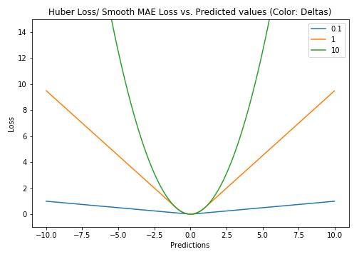
Huber Loss
Huber Loss is a combination of MAE & MSE. It is quadratic for smaller errors and linear otherwise i.e it acts like MSE for error closer to 0 and like MAE elsewhere. It is differentiable at 0 unlike MAE. How small that error has to be to make it quadratic depends on a hyperparameter, 𝛿 (delta). It approaches MAE when 𝛿 ~ 0 and MSE when 𝛿 ~ ∞.
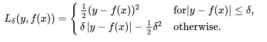
def huber(true, pred, delta):
    loss = np.where(np.abs(true-pred) < delta , 0.5*((true-pred)**2), delta*np.abs(true - pred) - 0.5*(delta**2))
    return np.sum(loss)
The downside being that we might need to train the hyper parameter 𝛿 (delta) which is an iterative process.
Log Cosh Loss
Log-cosh is the logarithm of the hyperbolic cosine of the prediction error.
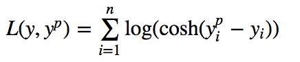
It acts like a quadratic loss for smaller values of x and a shifted version of abs(x) for larger values of x. It is also twice differentiable, which is very useful for methods like XGBoost which use Hessian matrix for optimisation.
def logcosh(true, pred):
    loss = np.log(np.cosh(pred - true))
    return np.sum(loss)
Classification Metrics
- Soft Labels - Classifier’s probability scores
- Hard Labels - Label associated with a prediction; usually argmax(soft_labels)
Matthews Correlation Coefficient
Matthews Correlation Coefficient

- Used for binary classification
- It is regarded as a balanced measure which can be used even if the classes are of very different sizes.
- MCC is in essence a correlation coefficient between the observed and predicted binary classifications
- A coefficient of +1 represents a perfect prediction (FP=FN=0),
0no better than random prediction and−1(TP=TN=0) indicates total disagreement between prediction and observation. - MCC is also perfectly symmetric, so no class is more important than the other; if you switch the positive and negative, you’ll still get the same value.
F1-Score
Precision

- Precision talks about how precise/accurate your model is out of those predicted positive, how many of them are actual positive.
- Precision is a good measure to use if the cost of false positive is high Eg. In a spam detector, if a non-spam mail is classified as spam, then the user might lose an important mail.
Recall
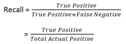
- Recall actually calculates how many of the actual positives our model capture through labeling it as Positive
- Recall is a good measure to use if the cost of false negative is high
Accuracy
- It is the fraction of correctly classified objects
- The best constant for accuracy => Always predicting the class with highest frequency
- Accuracy also doesn’t care how how confident the classifier is in the predictions i.e. it doesn’t care about the predicted class probabilities. It is harder to optimise and it only cares about the class labels.
- It is most used when all the classes are equally important.
Accuracy = (TP + TN) / (TP + TN + FP + FN)
LogLoss
- LogLoss cares about soft labels i.e. class probabilities. Log Loss takes into account the uncertainty of your prediction based on how much it varies from the actual label.
-
The probabilities always sum upto 1

-
M- number of possible class labels (dog, cat, fish) -
log- the natural logarithm -
y- a binary indicator (0 or 1) of whether class label c is the correct classification for observation o -
p- the model’s predicted probability that observation o is of class c
-
- LogLoss hugely penalises wrong answers as can be seen in the above graph (actual class=1). As we move towards the correct prediction the loss decreases & there’s an upward curve when we predict the class as 0
- Optimal Constant (LogLoss): Set probabilities as frequency of the classes. [0.1, 0.9] if number of class1 samples is 10 and number of class2 samples is 90.
AUC ROC
- Tries all possible values as threshold & then aggregates their scores.
- Used only for binary tasks. Depends on the ordering of predictions, not on absolute values.
- ROC is a probability curve and AUC represents degree or measure of separability.
- Random prediction leads to AUC = 0.5
AUC ROC Curve
- An ROC curve plots TPR vs. FPR at different classification thresholds. Lowering the classification threshold classifies more items as positive, thus increasing both False Positives and True Positives.
Pairs Ordering
- It is the ratio of correctly ordered pair upon total number of pairs. Ordering/Sorting of samples based on score is important.
- AUC is the probability that score for the false positive will be greater than the score for true positive.
AUC = # correctly ordered pairs / # total number of pairs
- Example - Suppose the ordering based on probability score is
[TP, FP, TP, TP, FP, FP]then there are $7$ instances/pairs when $score(FP) > score(TP)$ out of 9 possible pairs. So, AUC = 7/9- TP is when a model has correctly classified a sample as positive class
- FP is when a model has wrongly classified a sample as positive class
- TN is when a model has correctly classified a sample as negative class
- FN is when a model has wrongly classified a sample as negative class
Quiz
How would multiplying all of the predictions from a given model by 2.0 (for example, if the model predicts 0.4, we multiply by 2.0 to get a prediction of 0.8) change the model’s performance as measured by AUC?
No change. AUC only cares about relative prediction scores. AUC is based on the relative predictions, so any transformation of the predictions that preserves the relative ranking has no effect on AUC. This is clearly not the case for other metrics such as squared error, log loss, or prediction bias (discussed later).
LogLoss value for N number of classes with constant prediction.
log(N)
Cohen’s Kappa
The Kappa statistic (or value) is a metric that compares an Observed Accuracy with an Expected Accuracy (random chance). In addition, it takes into account random chance (agreement with a random classifier), which generally means it is less misleading than simply using accuracy as a metric.
The kappa statistic is often used as a measure of reliability between two human raters. In supervised learning, one of the raters reflects “ground truth”, and the other “rater” is the machine learning classifier.
Alternativey, since error=1 - accuracy,
Cohen’s Kappa ranges from [-1, 1]
Example
Assume Confusion Matrix for a binary classification task as follows
| Cats | Dogs | |
|---|---|---|
| Cats | 10 | 7 |
| Dogs | 5 | 8 |
Observed Accuracy
It is simply the number of instances that were classified correctly throughout the entire confusion matrix ie the number of instances when the ground truth and classifier both agreed to a particular class for a sample.
Total Number of Instances = 30 Observed Accuracy = (10+8 ) / 30 = 0.6
Expected Accuracy
Kappa
Quadratic Weighted Kappa
from sklearn.metrics import cohen_kappa_score, confusion_matrix
qwk = cohen_kappa_score(actuals, preds, weights="quadratic")
Target & Metric
- Target Metric is what we want to optimise. It is how the model is eventually evaluated.
- But no one really knows how to optimise target metrics efficiently. So, instead, we use Loss Functions, which is easy to optimise. Example it is not easy to optimise Accuracy Score, so we optimise for LogLoss & eventually evaluate our model using Accuracy Score.
- However, sometimes, the models can however optimise target metrics directly example MSE, LogLoss.
- Sometimes it is not possible to optimise target metric directly but we can somehow preprocess the train data and use a model with a metric or loss function which is easy to optimise. For example, optimising MSPE or MAPE is not easy, but we can instead optimise MSE
- Sometimes, we will optimise incorrect metrics but we will post-process to fit evaluation metric better
- A technique that always works is early stopping. Suppose that we have to optimise for M2, but cannot optimise directly. So, we instead optimise for metric M1 and monitor metric M2 on validation set. We stop when the model starts overfitting on M2.
Regression Metrics Optimization
MSE
Most of the libraries have MSE implemented as a loss function, so we can directly optimise for MSE. Synonyms - L2 Loss
- Tree-Based : LightGBM, RandomForest and XGBoost
- Linear-Model : SGDRegressor, Vowpal Vabbit
- Neural Nets : Pytorch, Keras, TF
MAE
MAE is another commonly used metric, so most of the libraries can optimise for MAE directly. Synonyms - L1 Loss, Quantile loss, Huber loss
- Tree-Based : LightGBM, RandomForest,
XGBoost - Neural Nets : Pytorch, Keras, TF
RMSLE
Train
- Transform the target
z = log(y+1)
- Fit a model with MSE loss
Test
- Transform the prediction probabilities back
y = exp(z) - 1
Classification Metrics Optimization
LogLoss
Similar to MSE in terms of popularity & hence implemented in almost all the major libraries.
- Tree-Based :- LightGBM and XGBoost
- Linear-Model :- SGDRegressor, Vowpal Vabbit
- Neural Nets :- Pytorch, Keras, TF
AUC
Optimise pairwise loss for optimising AUC
- Tree-Based :- LightGBM and XGBoost
- Neural Nets :- Pytorch, Keras, TF
F1-Score
def f1_metric(y_true, y_pred):
    y_pred = K.round(y_pred)
    tp = K.sum(K.cast(y_true*y_pred, 'float'), axis=0)
    tn = K.sum(K.cast((1-y_true)*(1-y_pred), 'float'), axis=0)
    fp = K.sum(K.cast((1-y_true)*y_pred, 'float'), axis=0)
    fn = K.sum(K.cast(y_true*(1-y_pred), 'float'), axis=0)

    p = tp / (tp + fp + K.epsilon())
    r = tp / (tp + fn + K.epsilon())

    f1 = 2*p*r / (p+r+K.epsilon())
    f1 = tf.where(tf.is_nan(f1), tf.zeros_like(f1), f1)
    return K.mean(f1)

def f1_loss(y_true, y_pred):

    tp = K.sum(K.cast(y_true*y_pred, 'float'), axis=0)
    tn = K.sum(K.cast((1-y_true)*(1-y_pred), 'float'), axis=0)
    fp = K.sum(K.cast((1-y_true)*y_pred, 'float'), axis=0)
    fn = K.sum(K.cast(y_true*(1-y_pred), 'float'), axis=0)

    p = tp / (tp + fp + K.epsilon())
    r = tp / (tp + fn + K.epsilon())

    f1 = 2*p*r / (p+r+K.epsilon())
    f1 = tf.where(tf.is_nan(f1), tf.zeros_like(f1), f1)
    return 1 - K.mean(f1)
Mean Encoding
- We encode each level of categorical variable with corresponding target mean.
- The more complicated and non linear is the feature target dependency more effective is mean encoding
- Greater the number of level in categorical features is a good indicator of using mean encodings
- Prone to overfitting if the levels in categorical features in train and test datasets are different
- Unlike other encoding techniques, mean encoding imposes an ordering
Ways to construct mean encoding
Possible Leaks
Calculate means only on the train data. Then calculate mean encodings using by applying map function on both the train & test data.
# col = categorical feature
# target = target column
means = X_train.groupby(col).target.mean()
train[col + '_mean_target'] = train[col].map(means)
val[col + '_mean_target'] = val[col].map(means)
Regularization
Expanding Mean
- Introduces least amount of leakage
- No hyper parameters to tune
- Built in CatBoost
cumsum = train.groupby(col)['target'].cumsum() - train['target']
cumcnt = train.groupby(col).cumcnt()
train_new[col+'_mean_target'] = cumsum/cumcnt
Regression
Encode your categorical variable with the mean of the target. For every category, you calculate the corresponding mean of the target (among this category) and replace the value of a category with this mean. More flexible compared to classification tasks as you can use a variety of statistics like median, standard deviations, percentiles, etc.